The Slow Death of Neoliberalism: Part 3 The Phillips Curve and Critical Theory
I described attacks on the Phillips Curve in Part 2. This part discusses the history of the Phillips Curve in detail, and concludes with a discussion of the problems revealed by the failure. The Observations are the fun part if this is too long.
History of the Phillips Curve
This section is based on parts 1-3 of The History of the Phillips Curve: Consensus and Bifurcation by Robert Gordon, an economist at Northwestern, published in the 2008 in the journal Economica at p. 10 et seq. (behind paywall, but available online through your local library). In 1958, William Phillips published a paper which as Gordon puts it,
… replaced discontinuous and qualitative descriptions by a quantitative hypothesis based on an unusually long history of evidence. Since 1861 there had been a regular negative relationship in Britain between the unemployment rate and the growth rate of the nominal wage rate. P. 12.
Phillips fitted a curve to data from the period 1861-1913, and plotted data for the remaining periods, through 1957 against that curve to find disagreements. Phillips found that his curve was close across the entire time except for a couple of years that he explains away. Here’s the curve Phillips fitted to his data:
1) wt = -.90 + 9.64U-1.39
Gordon says “… the inflation rate would be expected to equal the growth rate of wages minus the long-term growth rate of productivity.” P. 12.
1a) p = w – k
For some reason p is inflation and k is productivity. Upper case letters are levels and lower case letters are rates of change. So equation 1 can be written
2) p = -.90 + 9.64U-1.39 – k.
Paul Samuelson and Robert Solow discussed the Phillips results in the US context in a 1960 article. They found no similar data for the US, but they did some estimates and suggested that the PC doesn’t fit their data for several periods, and that it can shift up and down. Phillips estimated that an unemployment rate of about 2.5% was consistent with zero-inflation, while Samuelson and Solow think it might have been 3% pre-World War II and was about 5-6% in the early 60s.
With this seal of approval, the idea was incorporated into econometric models in two equations. In one, the PC was embodied and other variables were added, including demand, unemployment, the rate of change of unemployment, taxes, expected inflation and others in different combinations. This result was fed into an equation that calculates inflation based on wage levels, price levels and trend productivity. Gordon explains that
The reduced form of this approach implied that the inflation rate depended on the level and rate of change of unemployment, perhaps other measures of demand, and lagged inflation.
This is followed by a long discussion of the views of the Chicago School, which Gordon dismisses as utter failures. Moving along to 1975, Gordon turns to efforts to modify the Phillips Curve by adding supply and demand shocks. The price of oil shot up in 1973 because of OPEC. The demand for oil doesn’t decrease quickly in the short run, so people spend more on oil and less on other things. The Phillips Curve didn’t predict the results. Gordon says
The required condition for continued full employment is the opening of a gap between the growth rate of nominal GDP and the growth rate of the nominal wage to make room for the increased nominal spending on oil. P. 21, cite omitted.
That means wages must fall, Gordon says, or we have to add money to the economy, but the latter would lead to inflation. What we actually did, he says, was wage rigidity, increased unemployment, and some nominal (meaning not adjusted for inflation) GDP growth. Gordon then developed and published this version of the Phillips Curve:
3. pt = Ept + b(Ut – UtN) + zt + et
The second U term is the “natural” rate of unemployment, which I’m not going to take up. The z term represents cost-push pressure from unions and supply monopolies. The e term is apparently a constant but it seems odd that it might vary over time. Gordon explains that this version incorporates inertia, the idea that if there’s inflation in one period, there will be inflation in the next. It also reflects supply and demand issues, like wage and price rigidity.
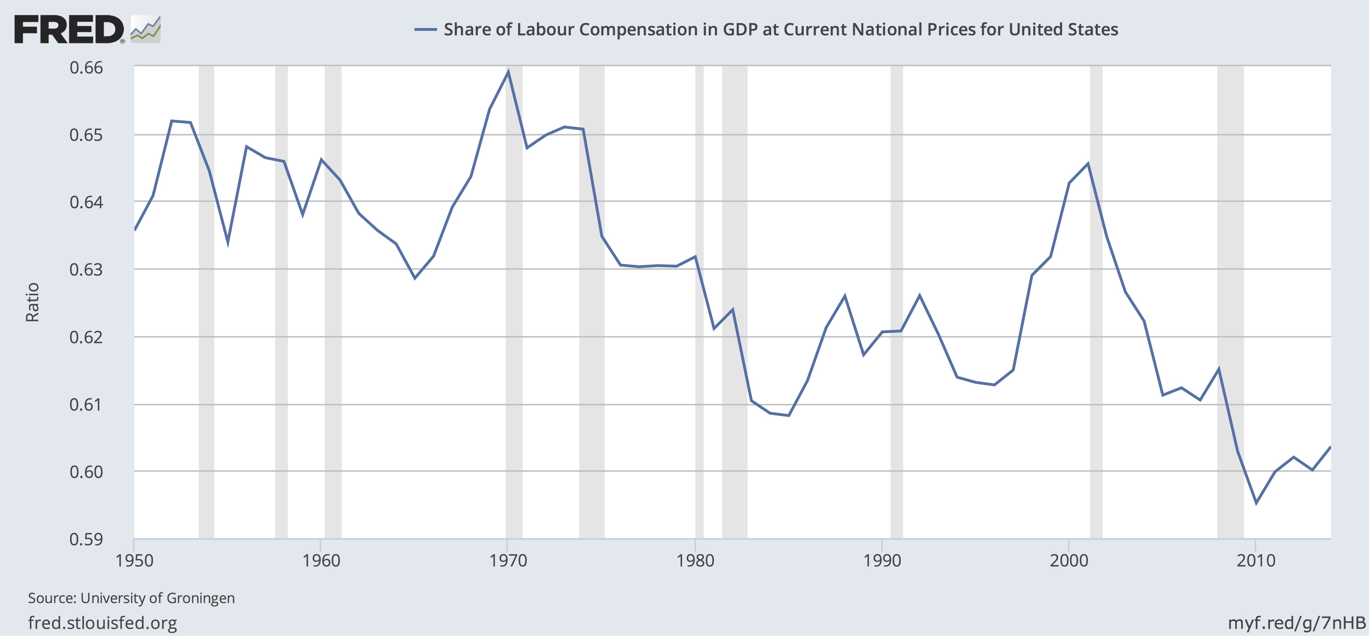
Gordon then mentions in passing that the wage equation (Equation 1a) is only valid if labor’s share of the GDP is fixed, but it isn’t. Here’s a chart from FRED

That problem, says Gordon, is “fruitfully ignored”. We don’t need to consider wages, we just look at prices. With these changes, we can understand the past by explaining away variations with negative or “beneficial supply shocks” and other variables. Gordon says that Equation 3 is foundation of the mainstream model. There is a related model, the New Keynesian Phillips Curve which is similar except that it incorporates future expectations of inflation, and makes no specific provision for supply and demand shocks. I assume these in some combination are the models used by the Fed, and heavily criticized as discussed in Part 2.
Observations
The concept is replaced by the formula, the cause by rules and
probability. Dialectic of Enlightenment, Horkheimer and Adorno,p. 3.
1. Phillips was working off empirical data when he fitted his curve, data about inflation and the rate of growth of wages. There are some theoretical issues in the preparation of that data. But the only abstract theory he adds to his data is Equation 1a, which Gordon says has a solid base in intuition. At the time he was writing, Phillips would only have seen data supporting that theory. We have new information:

As it happens, and perhaps not surprisingly, Phillips’ Equation 1 doesn’t work on US data. Gordon himself and others start adding things to make the Philips Curve work. They are convinced that there is a link between unemployment and inflation, and that they just need to add the relevant variables from their theoretical arsenal to get it to come out. Some focus on expectations, others on supply and demand shocks, and others add taxes or something else. Once they get those pesky variables set up, it’s just a matter of solving for constants. The point is to fit a curve to the actual data, not to use the actual data to see what’s happening. The concept connected to the real world is gone, replaced by the formula. The cause is replaced by the rules of economics.
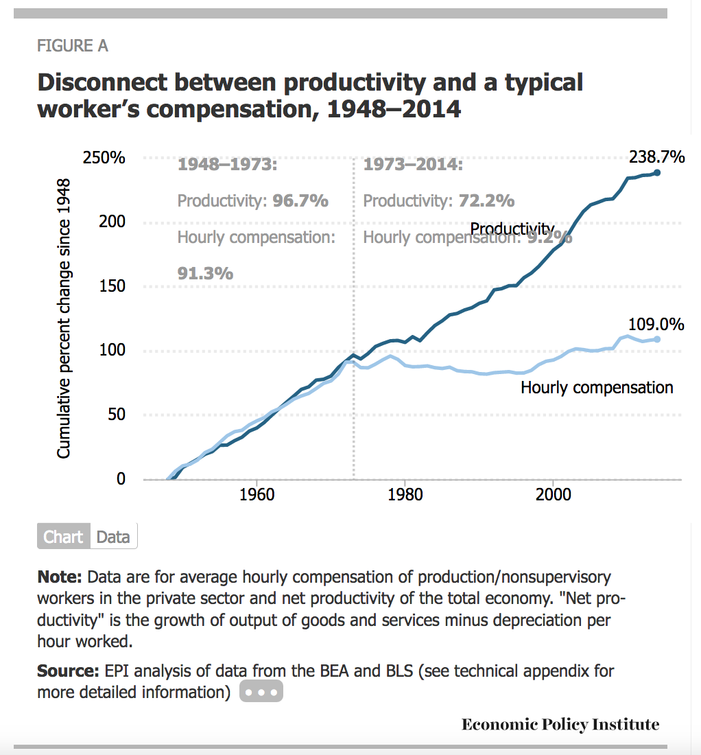
2. If we set inflation at 0 in Equation 1a, the rate of wage growth is equal to the rate of productivity growth. As the above chart shows, this relationship broke about 50 years ago. If all the gains from productivity are not going to labor, they are going to capital. Of course, capital takes several forms, for example, housing, agricultural land and other domestic capital. See, Piketty, Capital in the Twenty-First Century, Figure 4.6. When you think about it, it seems almost impossible that some of the gains from productivity weren’t going to capital all along. But in the current economy, it’s obvious that companies like Facebook can provide vastly more services with disproportionally fewer additional employees, few of whom are well paid, so that most of the gains from increased sales go to capital. Or, suppose that manufacturing is outsourced, reducing labor costs. Some of the gains might go to cutting prices but surely some go to capital. Let’s rewrite Equation 1a to reflect this, using γ for the growth rate capital.
1b) p = w + γ – k.
Using Equation 1b instead of 1a, we would have this instead of Equation 2:
4) p = -.90 + 9.64U-1.39 + γ – k.
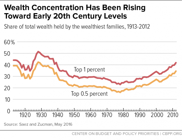
This equation focuses attention on the changes in the return to capital. That issue never seems to trouble most economists, but the rate of return to capital is the central focus of Piketty’s Capital In The Twenty-First Century. This chart from the Center on Budget and Political Priorities shows that top wealth started on its climb at the same time wages diverged from productivity, which supports the idea that gains from productivity are going to capital:

It also calls attention to the fact that nowhere in Gordon’s paper is there a mention of power, market power, political power, or social power, all of which Piketty talks about. Actually, hidden away in Gordon’s article is a backhanded reference to power. Equation 3 (Equation 7 in Gordon’s paper) includes a term “…zt to represent ‘cost-push pressure by unions, oil sheiks, or bauxite barons’”. P. 22. Obviously Gordon understands that the power to control the price of goods and services could create a negative supply shock, and the loss of control could produce a beneficial supply shock. P. 25. However, this is not explicit, and it certainly doesn’t deal with our current economy, in which almost all goods and services are dominated by a small number of gigantic companies exercising a significant degree of price control.
The tweaking Gordon describes might work for a while, but as the degree of price control through monopoly and oligopoly power increases, and γ becomes a bigger factor, the tweaks quit working.
3. Let’s put this in a larger context. For many economists, the Phillips Curve is structural. But why would you think so? It seems more likely that the relationship holds in a certain set of social conditions, including legislation and regulation, power conditions, and people’s attitudes. A logical use of the data is to work out the conditions that must exist to make it so. That’s how Piketty approaches his inequality data.
It’s a mistake to use a coincidence to predict the future. It seems to be a particular problem in economics. Even people who seem to know better continue to believe in the Phillips Curve. Here’s the President of the Boston Fed, Eric Rosengren:
A number of papers at the conference highlighted that some of the economic relationships that are frequently assumed to be stable over time have proven to be not so stable as we have come out of the financial crisis. These structural changes mean that if you tried to have a model that was fairly invariant to these changes, or a process that was invariant to these changes, there would start being big misses in monetary policy.
He goes on to explain that we have to raise interest rates because maybe not the Phillips Curve, but when employment goes up, inflation goes up. Rosengren knows there’s a problem, but he doesn’t have any idea of how to cope, so he keeps doing what he thinks he knows is right. It’s another example of Horkheimer and Adorno’s statement in action.
Updated to define γ more exactly.