Posts

The Slow Death of Neoliberalism: Part 3 The Phillips Curve and Critical Theory

Part 1.
Part 2.

I described attacks on the Phillips Curve in Part 2. This part discusses the history of the Phillips Curve in detail, and concludes with a discussion of the problems revealed by the failure. The Observations are the fun part if this is too long.

History of the Phillips Curve

This section is based on parts 1-3 of The History of the Phillips Curve: Consensus and Bifurcation by Robert Gordon, an economist at Northwestern, published in the 2008 in the journal Economica at p. 10 et seq. (behind paywall, but available online through your local library). In 1958, William Phillips published a paper which as Gordon puts it,

… replaced discontinuous and qualitative descriptions by a quantitative hypothesis based on an unusually long history of evidence. Since 1861 there had been a regular negative relationship in Britain between the unemployment rate and the growth rate of the nominal wage rate. P. 12.

Phillips fitted a curve to data from the period 1861-1913, and plotted data for the remaining periods, through 1957 against that curve to find disagreements. Phillips found that his curve was close across the entire time except for a couple of years that he explains away. Here’s the curve Phillips fitted to his data:

1) wt = -.90 + 9.64U-1.39

Gordon says “… the inflation rate would be expected to equal the growth rate of wages minus the long-term growth rate of productivity.” P. 12.

1a) p = w – k

For some reason p is inflation and k is productivity. Upper case letters are levels and lower case letters are rates of change. So equation 1 can be written

2) p = -.90 + 9.64U-1.39 – k.

Paul Samuelson and Robert Solow discussed the Phillips results in the US context in a 1960 article. They found no similar data for the US, but they did some estimates and suggested that the PC doesn’t fit their data for several periods, and that it can shift up and down. Phillips estimated that an unemployment rate of about 2.5% was consistent with zero-inflation, while Samuelson and Solow think it might have been 3% pre-World War II and was about 5-6% in the early 60s.

With this seal of approval, the idea was incorporated into econometric models in two equations. In one, the PC was embodied and other variables were added, including demand, unemployment, the rate of change of unemployment, taxes, expected inflation and others in different combinations. This result was fed into an equation that calculates inflation based on wage levels, price levels and trend productivity. Gordon explains that

The reduced form of this approach implied that the inflation rate depended on the level and rate of change of unemployment, perhaps other measures of demand, and lagged inflation.

This is followed by a long discussion of the views of the Chicago School, which Gordon dismisses as utter failures. Moving along to 1975, Gordon turns to efforts to modify the Phillips Curve by adding supply and demand shocks. The price of oil shot up in 1973 because of OPEC. The demand for oil doesn’t decrease quickly in the short run, so people spend more on oil and less on other things. The Phillips Curve didn’t predict the results. Gordon says

The required condition for continued full employment is the opening of a gap between the growth rate of nominal GDP and the growth rate of the nominal wage to make room for the increased nominal spending on oil. P. 21, cite omitted.

That means wages must fall, Gordon says, or we have to add money to the economy, but the latter would lead to inflation. What we actually did, he says, was wage rigidity, increased unemployment, and some nominal (meaning not adjusted for inflation) GDP growth. Gordon then developed and published this version of the Phillips Curve:

3. pt = Ept + b(Ut – UtN) + zt + et

The second U term is the “natural” rate of unemployment, which I’m not going to take up. The z term represents cost-push pressure from unions and supply monopolies. The e term is apparently a constant but it seems odd that it might vary over time. Gordon explains that this version incorporates inertia, the idea that if there’s inflation in one period, there will be inflation in the next. It also reflects supply and demand issues, like wage and price rigidity.

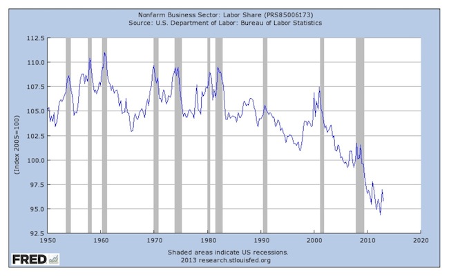
Gordon then mentions in passing that the wage equation (Equation 1a) is only valid if labor’s share of the GDP is fixed, but it isn’t. Here’s a chart from FRED

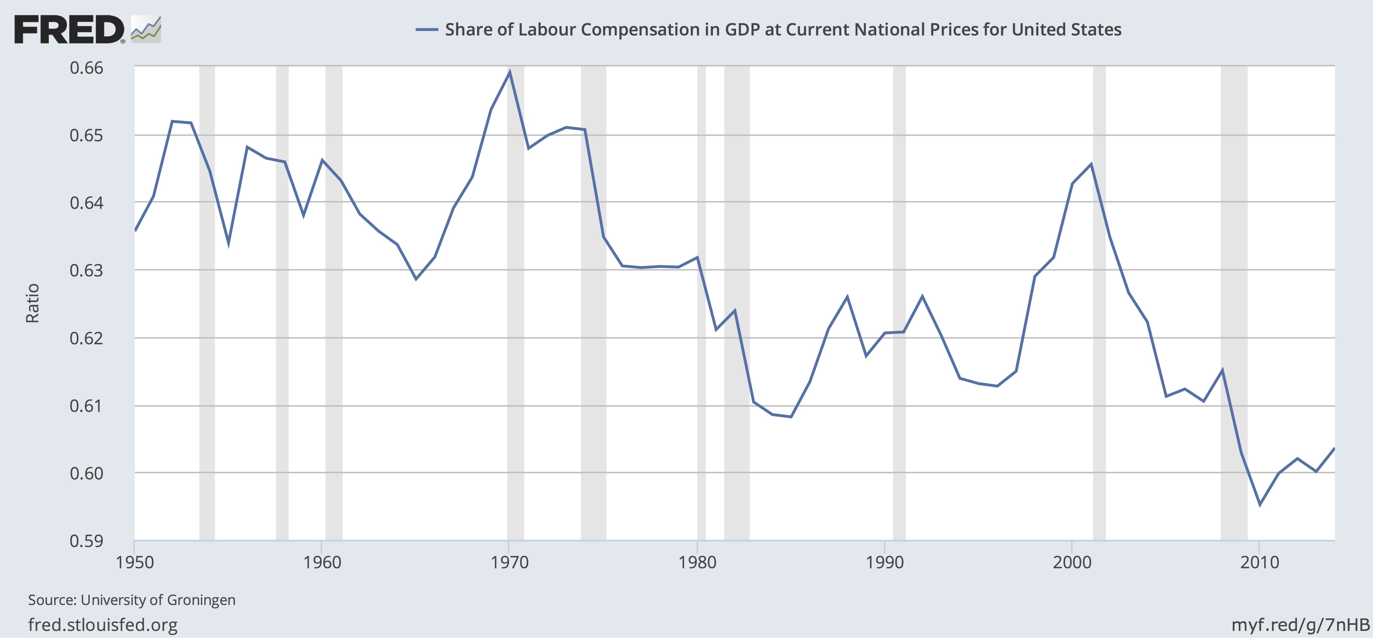
That problem, says Gordon, is “fruitfully ignored”. We don’t need to consider wages, we just look at prices. With these changes, we can understand the past by explaining away variations with negative or “beneficial supply shocks” and other variables. Gordon says that Equation 3 is foundation of the mainstream model. There is a related model, the New Keynesian Phillips Curve which is similar except that it incorporates future expectations of inflation, and makes no specific provision for supply and demand shocks. I assume these in some combination are the models used by the Fed, and heavily criticized as discussed in Part 2.

Observations

The concept is replaced by the formula, the cause by rules and
probability. Dialectic of Enlightenment, Horkheimer and Adorno,p. 3.

1. Phillips was working off empirical data when he fitted his curve, data about inflation and the rate of growth of wages. There are some theoretical issues in the preparation of that data. But the only abstract theory he adds to his data is Equation 1a, which Gordon says has a solid base in intuition. At the time he was writing, Phillips would only have seen data supporting that theory. We have new information:

As it happens, and perhaps not surprisingly, Phillips’ Equation 1 doesn’t work on US data. Gordon himself and others start adding things to make the Philips Curve work. They are convinced that there is a link between unemployment and inflation, and that they just need to add the relevant variables from their theoretical arsenal to get it to come out. Some focus on expectations, others on supply and demand shocks, and others add taxes or something else. Once they get those pesky variables set up, it’s just a matter of solving for constants. The point is to fit a curve to the actual data, not to use the actual data to see what’s happening. The concept connected to the real world is gone, replaced by the formula. The cause is replaced by the rules of economics.

2. If we set inflation at 0 in Equation 1a, the rate of wage growth is equal to the rate of productivity growth. As the above chart shows, this relationship broke about 50 years ago. If all the gains from productivity are not going to labor, they are going to capital. Of course, capital takes several forms, for example, housing, agricultural land and other domestic capital. See, Piketty, Capital in the Twenty-First Century, Figure 4.6. When you think about it, it seems almost impossible that some of the gains from productivity weren’t going to capital all along. But in the current economy, it’s obvious that companies like Facebook can provide vastly more services with disproportionally fewer additional employees, few of whom are well paid, so that most of the gains from increased sales go to capital. Or, suppose that manufacturing is outsourced, reducing labor costs. Some of the gains might go to cutting prices but surely some go to capital. Let’s rewrite Equation 1a to reflect this, using γ for the growth rate capital.

1b) p = w + γ – k.

Using Equation 1b instead of 1a, we would have this instead of Equation 2:

4) p = -.90 + 9.64U-1.39 + γ – k.

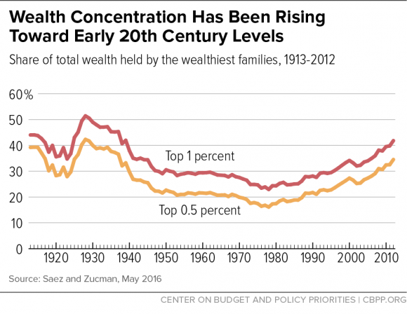
This equation focuses attention on the changes in the return to capital. That issue never seems to trouble most economists, but the rate of return to capital is the central focus of Piketty’s Capital In The Twenty-First Century. This chart from the Center on Budget and Political Priorities shows that top wealth started on its climb at the same time wages diverged from productivity, which supports the idea that gains from productivity are going to capital:

It also calls attention to the fact that nowhere in Gordon’s paper is there a mention of power, market power, political power, or social power, all of which Piketty talks about. Actually, hidden away in Gordon’s article is a backhanded reference to power. Equation 3 (Equation 7 in Gordon’s paper) includes a term “…zt to represent ‘cost-push pressure by unions, oil sheiks, or bauxite barons’”. P. 22. Obviously Gordon understands that the power to control the price of goods and services could create a negative supply shock, and the loss of control could produce a beneficial supply shock. P. 25. However, this is not explicit, and it certainly doesn’t deal with our current economy, in which almost all goods and services are dominated by a small number of gigantic companies exercising a significant degree of price control.

The tweaking Gordon describes might work for a while, but as the degree of price control through monopoly and oligopoly power increases, and γ becomes a bigger factor, the tweaks quit working.

3. Let’s put this in a larger context. For many economists, the Phillips Curve is structural. But why would you think so? It seems more likely that the relationship holds in a certain set of social conditions, including legislation and regulation, power conditions, and people’s attitudes. A logical use of the data is to work out the conditions that must exist to make it so. That’s how Piketty approaches his inequality data.

It’s a mistake to use a coincidence to predict the future. It seems to be a particular problem in economics. Even people who seem to know better continue to believe in the Phillips Curve. Here’s the President of the Boston Fed, Eric Rosengren:

A number of papers at the conference highlighted that some of the economic relationships that are frequently assumed to be stable over time have proven to be not so stable as we have come out of the financial crisis. These structural changes mean that if you tried to have a model that was fairly invariant to these changes, or a process that was invariant to these changes, there would start being big misses in monetary policy.

He goes on to explain that we have to raise interest rates because maybe not the Phillips Curve, but when employment goes up, inflation goes up. Rosengren knows there’s a problem, but he doesn’t have any idea of how to cope, so he keeps doing what he thinks he knows is right. It’s another example of Horkheimer and Adorno’s statement in action.

Updated to define γ more exactly.

The Slow Death of Neoliberalism: Part 2

The Slow Death of Neoliberalism Part 1.

This post focuses on the failings of neoliberal economic theory. Neoliberalism arises out of positivist philosophy, defined in Part 1. Positivism is the theory that the only true knowledge comes from the scientific process.

There are five main principles behind Positivism:

1. The logic of inquiry is the same across all sciences (both social and natural).

2. The goal of inquiry is to explain and predict, and thereby to discover necessary and sufficient conditions for any phenomenon.

3. Research should be empirically observable with human senses, and should use inductive logic to develop statements that can be tested.

4. Science is not the same as common sense, and researchers must be careful not to let common sense bias their research.

5. Science should be judged by logic, and should be as value-free as possible. The ultimate goal of science is to produce knowledge, regardless of politics, morals, values, etc.

Economists created a group of sayings which they put in their introductory textbooks and teach as laws and principles to their students at all levels. For example, N. Gregory Mankiw, economics professor at Harvard, starts his introductory economics textbook Principles of Macroeconomics with a list of ten Principles he claims almost all economists agree are true. Any thoughtful person reading this list will see that these ten statements are either tautological (you can’t do two things at once) or are mere rules of thumb. The idea that you could build a positivist science on this foundation is absurd. But Mankiw disagrees, and so does everyone who took Econ 101 and stopped, and especially so do the elites from our top schools.

It’s not surprising, then, that this version of economics is failing. It cannot perform the basic goal of a scientific theory, making accurate predictions. Economic models have failed and will continue to fail to predict disasters; and there isn’t much hope that they will ever be able to predict anything of interest.

In Part 1 I pointed out that the positivist program can’t be easily adapted to the social sciences. David Andolfatto of the St. Louis Fed agrees, and tells us what we can expect from economics:

But seriously, the delivery of precise time-dated forecasts of events is a mug’s game. If this is your goal, then you probably can’t beat theory-free statistical forecasting techniques. But this is not what economics is about. The goal, instead, is to develop theories that can be used to organize our thinking about various aspects of the way an economy functions. Most of these theories are “partial” in nature, designed to address a specific set of phenomena (there is no “grand unifying theory” so many theories coexist). These theories can also be used to make conditional forecasts: IF a set of circumstances hold, THEN a number of events are likely to follow. The models based on these theories can be used as laboratories to test and measure the effect, and desirability, of alternative hypothetical policy interventions (something not possible with purely statistical forecasting models).

This obvious straw man at the beginning of this quote is typical of the arrogant economist described by Marion Fourcade. But let’s see how well the economist business does at the weak test of effectiveness offered by Andolfatto.

For decades economists taught the Kuznets Curve which they said shows that as industrialization proceeds, economic inequality first rises and then falls.
Thomas Piketty takes up this theory in Capital In The Twenty-First Century, and extends the data forwards and backwards from the early 1950s. Here’s a graph of top decile income share from 1910 to 2010 from Wikipedia.

Looking at that graph through the time Kuznets wrote, the early 50s, it might be read to support that hypothesis. The sudden rise, starting under Reagan and continuing ever since, completely contradicts the hypothesis. That didn’t stop people from teaching it.

The Phillips Curve asserts that there is a connection between inflation and unemployment: as the unemployment rate drops, inflation increases. It’s one of Mankiw’s 10 principles; and it’s deeply embedded in the models used by the Fed to decide interest rates. It’s mostly wrong. Here’s a recent debunking from the Philadelphia Fed, concluding that the Phillips Curve might help forecast inflation in a weak economy, but does not work in an expanding economy.

The Wikipedia Page for Phillips Curve says that:

The original Phillips curve literature was not based on the unaided application of economic theory. Instead, it was based on empirical generalizations. After that, economists tried to develop theories that fit the data.

A 2008 paper, The History of the Phillips Curve: Consensus and Bifurcation, Economica (2008), P. 10, lays out the history in detail. Roughly speaking, it begins with the observation by William Phillips that in the UK there was a stable relation between the rate of wage growth and inflation over a substantial period of time, and deviations could be explained reasonably. This paper was picked up by Paul Samuelson and Robert Solow and turned into the earliest mathematical formula in 1958. Since then there have been a number of occasions where the Phillips Curve failed, and each time economists just grab some more of their existing tools and try to fix it or explain the failure, in each case after policy-makers have gone on as if it were right and forced bad results on the economy and especially the wages of workers.

Here’s a third example. Economists say that the reason wages are stagnant is that productivity is flat, as if there were a relation between wages and productivity. Anyone who looks at this chart and reads this article from the Economic Policy Institute will have a huge question about that.

And that isn’t just the right-wing. Plenty of centrist Democrats make the same argument. And by the way, what does this say about the central theory of free market economics that supply and demand for labor set prices?

As I say here and here, neoliberal economists used their ideology of free markets to influence policy and to change the entire way we think about society without having the slightest idea of the consequences of their meddling because their models aren’t designed to deal with changes in societies or economies. As my examples show, they just keep on regardless of the success or failure of their predictions, and politicians and rich people ignore the failings and continue to follow their foolish advice.

Neoliberal economics obviously fails to measure up to the standards of positivism. It can’t predict anything useful, and it barely is able to explain itself coherently. That’s a problem with positivism too. People are slowly, slowly coming to grips with these failures and the damage they have done. It’s adherents are dying off, and their replacements are into it for the money and the power. Stupid ideas never die, but maybe they will lose their influence.

Updated to correct link to EPI article and chart.

Mankiw’s Tenth Principle: Society Faces A Short-Run Trade-off Between Inflation and Unemployment

The introduction to this series is here.
Part 1 is here.
Part 2 is here.
Part 3 is here.
Part 4 is here.
Part 5 is here.
Part 6 is here.
Part 7 is here.
Part 8 is here.
Part 9 is here.

Mankiw’s tenth principle of economics is: Society faces a short-run trade-off between inflation and unemployment. He admits that this is more controversial among economists than his other principles. He says that most believe this explanation:

  • Increasing the amount of money in the economy stimulates the overall level of spending and thus the demand for goods and services.
  • Higher demand may over time cause firms to raise their prices, but in the meantime, it also encourages them to hire more workers and produce a larger quantity of goods and services.
  • More hiring means lower unemployment.

This line of reasoning leads to one final economy-wide trade-off: a short-run trade-off between inflation and unemployment.

This gives economic policy-makers a tool for influencing economic trends. “By changing the amount of money it prints”, says Mankiw, government can put more or less money into the economy, and thus influence unemployment, at least in the short run. The Great Crash of 2008 is an example. Mankiw explains that it was caused by “bad bets on the housing market”, and led to high unemployment and lower incomes. The Obama administration responded with a stimulus package of spending and tax cuts, and the Fed increased the amount of money in the economy, in an effort to reduce unemployment. He adds: “Some feared, however, that these policies might over time lead to an excessive level of inflation.”

The frightened people were, of course, proven absolutely wrong, though they won the policy argument with the imposition of the Sequester. The stimulus package was too small, though at least it more or less happened, and of course spending on the military increased, which helped, though it would have been nice to have something for the money besides the worthless F-35. This discussion is fleshed out beginning at about page 490 (in the 6th Ed.) with a long discussion of the Phillips Curve. This Wikipedia entry is at least cheaper than buying Mankiw’s book. for those not familiar with the subject.

This isn’t so much a principle in the sense of an axiom as it is a theorem, worked up from axioms. The source of the idea is a 1958 paper by William Phillips, showing an historical correlation between inflation and unemployment in the UK, and extended to US data by Paul Samuelson and Robert Solow. The correlation and the explanation worked together to persuade people that both the grounds of explanation and the relationship were more or less permanent features of the economy. The ideas behind the explanation are neoclassical, so the correlation served to validate those neoclassical ideas.

Recently the Wall Street Journal published an essay by Ben Leubsdorf discussing the current understanding of the Phillips Curve debate: The Fed Has a Theory. Trouble Is, the Proof Is Patchy. [Paywall]. Jared Bernstein discusses it in this post and links to this New York Times post; both are worth reading to see just how unhinged we are from the simple explanation offered by Mankiw. This chart is from the WSJ article.

Phillips Curve Chart 3

To read the chart, select an expansion, find the line in that color, and look for the circle, which is the beginning of the period. Then follow the line as it moves showing the changes in inflation (y-axis) and unemployment (x-axis). Here’s Leubsdorf’s explanation:

But the simple link between U.S. unemployment and inflation described by the Phillips curve appeared to break down after the 1960s. High inflation coexisted with high unemployment in the 1970s. In the 1990s, the jobless rate fell as price pressures weakened. Over the past three years, inflation has declined despite a falling jobless rate.

Mankiw says there is dispute among economists about this, and Leubsdorf confirms that. He says that a recent WSJ survey found that 2/3 of economists “believed that the link exists.” Here’s a quote from a believer, Atlanta Fed President Dennis Lockhart.

“In the absence of direct evidence that inflation is in fact converging to the target and in the absence of compelling or convincing direct evidence, I think a policy maker has to act on the view that the basic relationship in the Phillips curve between inflation and employment will assert itself in a reasonable period of time as the economy tightens up ….

Economists are fully aware of the problems with the Phillips Curve, and there are plenty of attempts to make it better. This is from the conclusion of an April 2015 Working Paper by Laurence Ball and Sandeep Mazumder of the International Fund:

One of Mankiw’s (2014) ten principles of economics is, “Society faces a short-run tradeoff between inflation and unemployment.” This tradeoff, the Phillips curve, is critically important for monetary policy and for forecasting inflation. It would be extraordinarily useful to discover a specification of the Phillips curve that fits the data reliably. Unfortunately, researchers have repeatedly needed to modify the Phillips curve to fit new data. Friedman added expected inflation to the Samuelson-Solow specification.

Subsequent authors have added supply shocks (Gordon, 1982), time-variation in the Phillips-curve slope(Ball et al., 1988), and time-variation in the natural rate of unemployment (Staiger et al.,1997). Each modification helped explain past data, but, as Stock and Watson (2010) observe, the history of the Phillips curve “is one of apparently stable relationships falling apart upon publication.” Ball and Mazumder (2011) is a poignant example.

Even today people are looking for a way to find something useful in past data to predict future outcomes. As Leubsdorf noted, the Fed is using some version of this curve in deciding when to raise interest rates.

So, how does this fit with neoliberalism? One of the goals of neoliberal economics is the protection of established wealth. Inflation erodes wealth. Returns to capital may or may not keep up with inflation, depending on the strength of labor and other factors of production. Debtors are able to repay their debt in less valuable dollars, which erodes the assets of creditors. If the increased returns are less than the erosion, wealth suffers. As we have seen in the wake of the Great Crash, the governing power structure of neoliberalism demands that capital be protected whether in the form of equity or debt. This principle tells policy makers to put people out of work rather than suffer inflation.

The Fed follows this principle. This is a chart of the labor share of income.
labor share 1
The gray vertical bars are recessions. The chart shows that as the labor share rises, we get a recession. The following chart shows bank prime rates.
Bank Prime Rate
As interest rates rise, we get recessions. With the exception of the recession that followed the Great Crash, it’s fair to say that all of these recessions were engineered by the Fed because of inflation or fear of inflation.

The implications are fascinating. Before the Great Crash, almost all US money was created by bank lending and credit expansion. Mankiw’s Principle No. 9 tells us that when too much money is created, we get inflation. The Phillips Curve tells the Fed it has to raise interest rates to stem inflation, and that it does so at the cost of putting people out of jobs. So, businesses lend and borrow too much, creating inflation or fear of inflation, and to solve the problem created by the failure of capitalists, the Fed makes sure only the working people pay the price, by losing their livelihoods, and lately, by watching their incomes stagnate or drop. And that is the outcome of applying Mankiw’s Principles of Economics: damaging workers to protect the rich.